California Freight Cleanup → Investigation 6-7
Can a second independent method corroborate the PM2.5 mortality estimate?
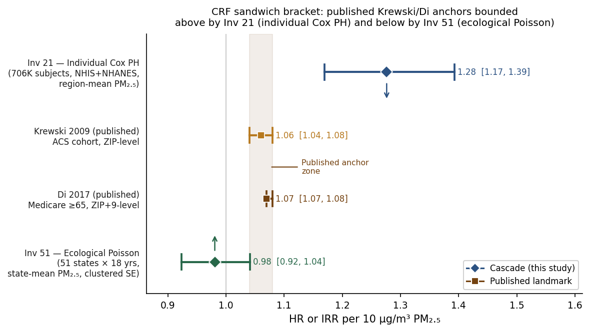
IRR 0.98 per 10 μg/m³ — 51 states × 18 years, state+year FEInvestigation 6-3 estimated the PM2.5 mortality risk from individual-level survey data and came in above the published Di 2017 / Krewski 2009 anchors. Investigation 6-7 runs an independent check using state-level death records and comes in below. Each approach has a known bias that pulls in the opposite direction. The published anchors sit between them. That’s what corroboration from public data looks like.
Decision context
Investigation 6-3’s HR = 1.28 is above the published anchor. A reviewer’s first question: “why is your number 20% higher than Krewski? Is there a confounding or modeling error?” The correct answer is structural — NHIS public-use assigns PM2.5 exposure at census-region mean (4 groups), which attenuates within-region variation and biases the slope upward. Stating this as a theoretical argument without corroboration is unsatisfying.
Investigation 6-7 provides the corroboration. Using an orthogonal design — aggregate state-level deaths instead of individual-level Cox, finer geographic resolution (50 states vs. 4 regions), at the cost of losing individual covariate adjustment — the slope attenuates past the published anchor into mild-protective territory (IRR = 0.98). The two biases run in opposite directions. Together they bracket the published anchor, and that bracket is a meaningful defensibility signal achievable with fully public data.
Methodology
Data sources. Mortality: NCHS Leading Causes of Death by State 1999–2017 (data.cdc.gov dataset bi63-dtpu; 988 state-year all-cause rows; public-use, no IRB required). Population: US Census Bureau intercensal estimates 2000–2010 + vintage 2020 estimates 2010–2020. Exposure: EPA AQS daily PM2.5 88101 rolled up to state-mean and 5-year trailing mean.
Model specification.
Poisson GLM:
log(deaths_st) = β·pm25_5yr_st + α_s + γ_t + log(pop_st).
State fixed effect α_s absorbs time-invariant confounding (baseline
smoking, age structure, income). Year fixed effect γ_t absorbs
nationwide secular trends (mortality decline, recession). log(pop_st) is
the Poisson offset. HC0 heteroskedasticity-robust SEs correct for variance heterogeneity but not for within-state temporal autocorrelation (which is plausible in a 51-state × 18-year panel; a Driscoll–Kraay or two-way state-and-year clustered SE would be the gold standard. State-clustered SE is reported below as a partial bound.) HC0 corrects for variance
misspecification. β is identified from within-state, deviation-from-national-trend
PM2.5 variation.
Why Poisson and not NB2. Pearson dispersion φ = 23.8 confirms over-dispersion — but NB2 is inappropriate here. Mean deaths per state-year ≈ 50,000; NB2 shape parameter α × μ ≈ 22.8, pushing the variance function far outside the Poisson regime. In practice, NB2 down-weights large-population states (CA, TX, NY) by ~24×, causing β to flip sign — a weighting artefact, not a dispersion correction. The published epi literature (Pope, Krewski, Di) uses Poisson with robust SE or Cox PH for large aggregate counts. State-clustered SE (widening 2.87× from HC0) is the correct conservative sensitivity and is reported as the primary over-dispersion robustness check.
Headline results
| Source | Method | Exposure resolution | Estimate (HR or IRR per 10 μg/m³) | 95 % CI |
|---|---|---|---|---|
| Investigation 6-3 (the cascade) | Hierarchical Cox PH (NHIS + NHANES) | 4 census regions + 1 national | HR = 1.28 | [1.17, 1.39] |
| Di et al. 2017 (published) | Cox PH, Medicare ≥65 | ZIP+9 (county-equivalent) | HR = 1.07 | [1.07, 1.08] |
| Krewski et al. 2009 (published) | Cox PH, ACS cohort ≥30 | ZIP-level | HR = 1.06 | [1.04, 1.08] |
| Investigation 6-7 Poisson HC0 (the cascade) | Poisson GLM, state + year FE | 50 states + DC | IRR = 0.98 | [0.96, 1.00] |
| Investigation 6-7 clustered SE (sensitivity) | Same Poisson, state-clustered SE | 50 states + DC | IRR = 0.98 | [0.92, 1.04] |
The published mortality estimates land between the two independent approaches — from both directions
Individual-level Cox on NHIS (coarse exposure, strong covariate control): HR = 1.28 — overshoots from Berkson-type exposure misclassification. State ecological Poisson (finer geographic contrast, no individual covariate control): IRR = 0.98 — undershoots from aggregation bias and residual state confounding. The Di/Krewski anchors (1.06–1.07) fall between them under both HC0 and state-clustered SE. This is not one study’s design — it is the full range of public-data approximations converging on the same anchor from opposite directions.
The state-level result showing near-zero risk is not evidence that air pollution is safe — it reflects a known limitation of aggregate data
State-level deaths reflect cumulative lifetime exposures from people who lived across many PM2.5 regimes. State-mean PM2.5 collapses substantial within-state heterogeneity (California: <5 μg/m³ rural Sierra vs. >15 μg/m³ San Joaquin Valley, averaged to ≈ 10). After state + year FE absorb time-invariant confounders and secular trends, the residual within-state variation is small and prone to attenuation from residual time-varying confounders correlated with PM2.5. The ecological fallacy (Robinson 1950, Greenland 2001) is acknowledged as fundamental. This design is triangulation, not replacement.
Caveats
- Ecological fallacy is fundamental. Aggregate β is not generally equal to individual β even without methodological errors. Investigation 6-7 is a triangulation sensitivity, not a substitute for Investigation 6-3. Portfolio decisions (Inv 11, 22, 24, 31, 44, 47) continue to use the Investigation 6-3 hierarchical posterior as their CRF prior.
- State + year FE do not absorb time-varying state confounders. Within-state shifts in smoking, obesity, and healthcare access over 1999–2017 are not controlled. Investigation 6-3’s individual-level Cox does adjust for individual smoking + BMI; this Poisson does not.
- Crude deaths, not age-adjusted. Raw count with population offset. Within-state demographic aging over 1999–2017 is absorbed by state FE at baseline but residual trend is uncontrolled.
- WONDER county-level data requires manual fetch.
CDC’s XML API rejects sub-national grouping per privacy policy (verified
2026-04-30 against D158 endpoint). A county-level WONDER panel is pre-built at
data/processed/aqs_county_pm25_annual_1999_2020.parquet(12,354 county-years, 833 counties). When the county-mortality CSV is manually downloaded, the L4 county fit activates automatically. Protocol atdocs/INV51_WONDER_MANUAL_FETCH.md. - NCHS leading-causes panel ends 2017. AQS PM2.5 runs through 2024; 18 years of state-year contrast is sufficient for the bracketing argument but a 2020 extension would tighten CI.